Methods
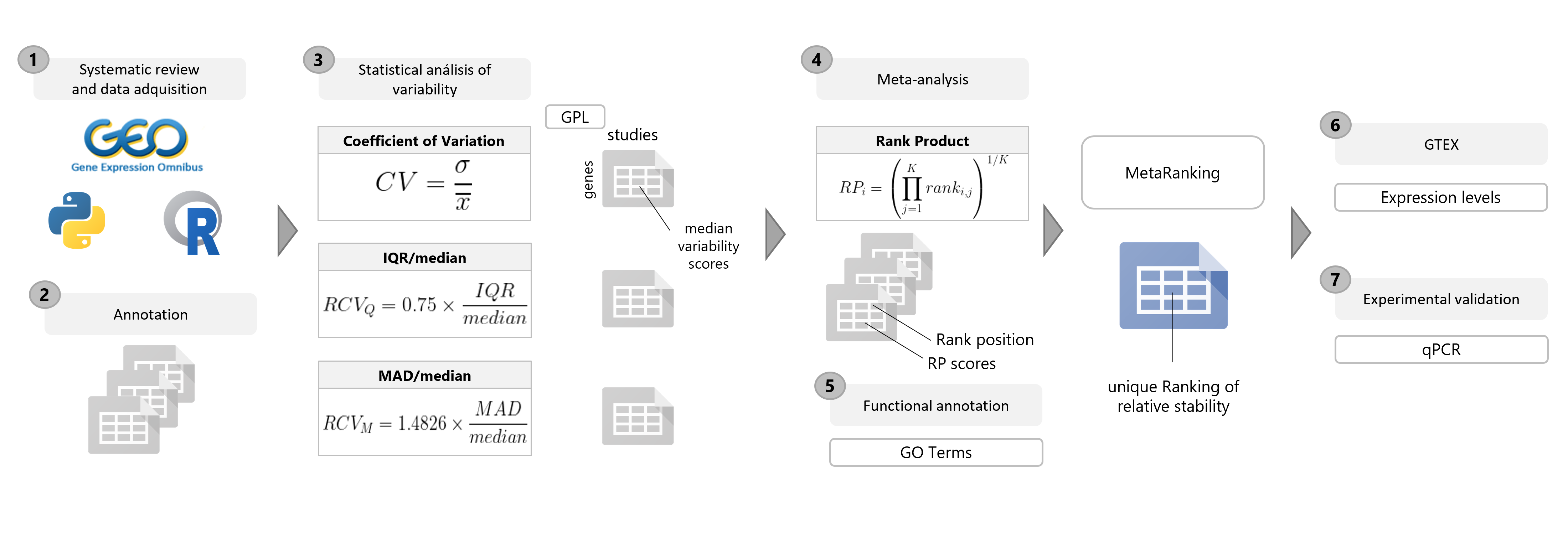
Bioinformatics and statistical analysis were run in R software v.3.5.0 [1]. Figure 1 summarizes the workflow followed in this study.
1. Systematic review and collection
1.1 Literature review
A comprehensive systematic review was conducted to identify all available transcriptomics studies with adipose tissue samples at GEO. The review considered the fields: sample source (adipose) type of study (expression profiling by array), and organism of interest (Homo sapiens or Mus musculus). The search was carried out during the first quarter of 2020, with the review period covering the years 2000-2019. From the returned records, the study GSE ID, the platform GPL ID, and the study type were extracted using the Python 3.0 library Beautiful Soup. The R package GEOmetadb [2] was then used to identify microarray platforms and samples from adipose tissue. The top 4 and 5 most used platforms in Hsa (Analysis Summary, Human Platform summary) and Mmu (Analysis Summary, Mouse Platform summary), respectively, were selected. Given the complex nature of some of the studies, those with information regarding the sex of samples were manually determined, and the keywords used to annotate them homogenized. Finally, studies not meeting the following predefined inclusion criteria were filtered out:
- include at least 10 adipose tissue samples
- use one of the selected microarray platforms to analyze gene expression data
- present data in a standardized way
- not include duplicate sample records (as superseries).
2. Data Processing and Statistical Analyses
The normalized microarray expression data of the selected studies from GEO were downloaded using the
GEOQuery R package. All the probe sets of each platform were converted to gene symbols, averaging
expression values of multiple probe sets targeting the same gene to the median value.
Three statistical stability indicators were calculated for each gene in each study to determine the
relative expression variability: the coefficient of variation (CV), the IQR/median, and the MAD/median.
The CV, computed as the standard deviation divided by the mean, is used to compare variation between
genes with expression levels at different orders of magnitude; however, extreme values can affect this
value. Therefore, the interquartile range (IQR) divided by the median and the median absolute deviation
(MAD) divided by the median (two statistics based on the median) were also considered. These measures
provide more robustness in skewed distributions [3]. Both statistics were multiplied by a correction
factor of 0.75 and 1.4826 to make them comparable to the CV in normal distributions. Lastly, the gene
variability scores per platform were expressed as the median of all statistics from the studies analyzed
with each platform. These median values were ranked by gene variability value for each platform, with
lower ranks corresponding to higher stability levels.
The described analysis pipeline was performed on three three different sample groups based on sex and
species: female Hsa, male Hsa, and all Mmu samples. The analysis was not performed separately for male
and female mice due to the lack of female Mmu samples.
3. Meta-analysis
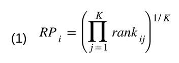
The gene variability ranks per for each platform were integrated using the Rank Product (RP) method [4,5], a
non-parametric statistic identifying the elements that systematically occupy higher positions in ranked
lists. This approach combines gene ranks rather than variability scores to create platform independence.
The RankProd package [6,7] was used to calculate the RP score for each gene (Equation 1, where i is the
gene, K the number of platforms, and rankij the position of gene i in the ranking of platform j). Three
final rankings were obtained (one for each sample group [Mmu, Hsa female, and Hsa male samples]) by
sorting the genes in increasing order of RP.
4. Selection of Candidate HKGs
To encounter appropriate suHKG candidates, male and female Hsa samples were randomly selected, and the
Mmu group was discarded. Gene functional information was then incorporated to exclude genes involved in
metabolic alterations. The AnnotationDbi and org.Hs.eg.db annotation packages converted Gene Symbol to
Gene name. After removing pseudogenes and non-coding genes, the associated GO terms of the remaining
genes were obtained using the GO.db annotation package. Related information from all three gene
ontologies were included (Biological Process, Molecular Function, Cellular component). Genes related to
physiopathological conditions were filtered out, and a unique ranking by sex was generated (the male and
female MetaRankings), which averages the three statistical rankings (Equation 2).

The difference in the ranking positions occupied in by males and females was also calculated to reveal
sex-based stability differences at a gene level.
Selecting stable suHKG with high levels of expression, followed several steps:
- Download the GTEx_Analysis_2017-06-05_v8_RNASeQCv1.1.9_gene_median_tpm.gct.gz file from GTEx,
- Select the adipose tissue samples,
- Take the gene median transcript per million (TPM) value in visceral adipose tissue.
- Filter out from our sex-specific MetaRankings genes with median TPM < 20.
- Select the genes in the top 10% positions of each MetaRanking.
- Intersect the two top lists to find stable and highly expressed genes common to both sexes.
5. Experimental validation
5.1 Study Selection and Sample Processing
Subjects were recruited by the endocrinology and surgery departments at the University Hospital Joan XXIII (Tarragona, Spain) in accordance with the Helsinki declaration. Visceral and subcutaneous adipose tissue samples were obtained during surgery from lean and obese male and female individuals. Total RNA was extracted from adipose tissue using the RNeasy lipid tissue midi kit (Qiagen Science). One microgram of RNA was reverse transcribed with random primers using the reverse transcription system (Applied Biosystems)33. Mouse adipose tissue was obtained from wild type and Irs2-/- [8] (insulin resistance and type 2 diabetes model) C57BL/6 littermates. According to the criteria outlined in the "Guide for the Care and Use of Laboratory Animals," all animals received humane care22. Total RNA was extracted from abdominal fat using a combined protocol including Trizol (Sigma) and RNeasy Mini Kit (Qiagen) with DNaseI Digestion. First-strand synthesis was performed using EcoDry Premix (Takara).
5.2. Gene Expression Analysis
Quantitative gene expression analysis was performed on 50 ng cDNA template. Real time-PCR was conducted in a LightCycler 480 Instrument IIR (Roche) using SYBR PreMix ExTaqTM (mi RNaseH Plus, Takara). Primers used in this study are noted in Table S4. Crossing point (Cp) values were analyzed for stability between samples and relative quantification using 2^-ΔCt. Statistical analyses were performed with GraphPad Prism 8 (Graphpad Software V 8.0). The results are expressed as arithmetic mean ± the standard error of the mean (SEM). When two data sets were compared, a Student's t-test was used. The differences observed were considered significant when: p-value < 0.05 (*), p-value < 0.01 (**) and p-value < 0.001 (***).
References
- R Core Team R: A Language and Environment for Statistical Computing; R Foundation for Statistical Computing: Vienna, Austria, 2019.
- Zhu Y, Davis S, Stephens R, Meltzer PS, Chen Y. GEOmetadb: powerful alternative search engine for the Gene Expression Omnibus. Bioinformatics. 2008;24(23):2798-2800. doi:10.1093/bioinformatics/btn520 .
- Arachchige C, Prendergast L, Staudte R. Robust analogs to the coefficient of variation. J Appl Stat. Published online August 20, 2020:1-23. doi:10.1080/02664763.2020.1808599.
- Breitling R, Armengaud P, Amtmann A, Herzyk P. Rank products: a simple, yet powerful, new method to detect differentially regulated genes in replicated microarray experiments. FEBS Lett. 2004;573(1-3):83-92. doi:https://doi.org/10.1016/j.febslet.2004.07.055.
- Mitchell L. A parallel implementation of the Rank Product method for R. :12.
- Hong F, Breitling R, McEntee CW, Wittner BS, Nemhauser JL, Chory J. RankProd: a bioconductor package for detecting differentially expressed genes in meta-analysis. Bioinformatics. 2006;22(22):2825-2827. doi:10.1093/bioinformatics/btl476.
- Del Carratore F, Jankevics A, Eisinga R, Heskes T, Hong F, Breitling R. RankProd 2.0: a refactored bioconductor package for detecting differentially expressed features in molecular profiling datasets. Bioinformatics. 2017;33(17):2774-2775. doi:10.1093/bioinformatics/btx292.
- Withers DJ, Gutierrez JS, Towery H, et al. Disruption of IRS-2 causes type 2 diabetes in mice. Nature. 1998;391(6670):900-904. doi:10.1038/36116