MetaEnrichGO Usage Instructions
This comprehensive tutorial explains how to use MetaEnrichGO, a Shiny-based tool for meta-analysis of functional enrichment across multiple gene lists. It covers all aspects from data input to the statistical methodology and result interpretation.
- Overview
- Inputs
- Input Methods
- Input Example
- Parameters
- Database
- Ontology (GO only)
- Personalized File Upload (Personalized only)
- Organism
- Gene ID Type
- Meta-Analysis Method
- Minimum Number of Datasets
- Data Visualization
- Table Columns
- Plot Settings
- Outputs
- Results Table
- Excluded Terms
- Plot Output
- Dotplot
- Barplot
- Results Table
- Background Pipeline
- Best Practices
- Troubleshooting
1 Overview
MetaEnrichGO facilitates functional enrichment analysis for lists of genes derived from meta-omics experiments. Its key features include:
- Multiple input modes (
upload,paste,example data). - Selection of functional databases: Gene Ontology (GO), Kyoto Encyclopedia of Genes and Genomes (KEGG), Reactome and Personalized Annotations.
- Support for several gene ID (
SYMBOL,ENTREZIDandENSEMBL) types and multiple organisms (Homo sapiens, Mus musculus and Rattus norvegicus). - Application of different p-value combination methods (
Fisher,Stouffer,Tippett,Wilkinson). - Visualization through interactive tables and plots.
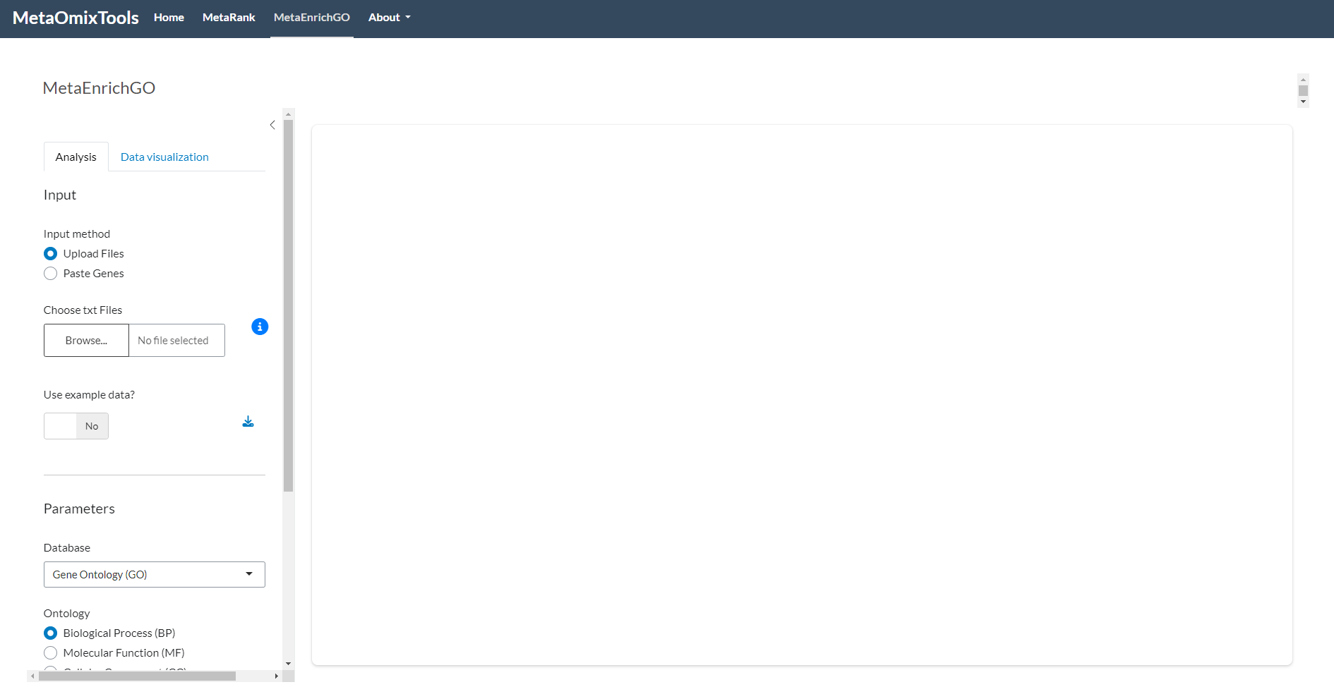
Figure 1: MetaEnrichGO Interface Overview. General view of the application dashboard highlighting input options, database selection, and analysis settings.
2 Inputs
2.1 Input Methods
Upload Files: When the “Upload Files” mode is enabled, it is possible to select one or more text files (
.txt) via the file upload control. The system recognizes each file as a list of genes (one identifier per line, without a header), automatically removes duplicates and missing values, and correctly handles both Unix (\n) and Windows (\r\n) line endings. If more than one gene is provided on a single line separated by delimiters (e.g.,BRCA1///BRCA2), only the first entry (BRCA1) is retained. Clicking the ℹ️ icon opens a modal showing a sample file structure, and example datasets can be downloaded for in-depth study and reference. There is no strict limit to the number of gene lists that can be uploaded, provided the total file size does not exceed 30 MB. The capacity depends on the size of each list; for example, when lists contain approximately 20,000 genes, up to 12 have been successfully processed. In contrast, for smaller lists (ranging from 100 to 500 genes), the system has handled up to 50 lists without issue.Paste Genes: When the “Paste Genes” mode is enabled, gene lists can be entered directly into a text area. Each list is delimited by
###, and within each section the system expects one gene per line (e.g.,TP53\nBRCA1\nEGFR), with no header row. Duplicate entries and blank lines are cleaned up automatically, and if a line contains multiple gene identifiers (e.g.,BRCA1///BRCA2), only the first is used. The placeholder text illustrates this formatting.Use Example Data: Enabling the “Use Example Data” switch loads predefined files that represent various analysis scenarios, allowing users to explore the workflow without providing their own data.
Note
Many elements in the interface include helpful tooltips that appear when you hover your mouse over them. These tooltips provide additional explanations, usage instructions, or data source information. For example, hovering over the Use Example Data switch reveals the origin of the example datasets, while the text input area for pasted genes displays detailed formatting guidance. Take advantage of these tooltips to better understand each parameter and improve your experience with the application.
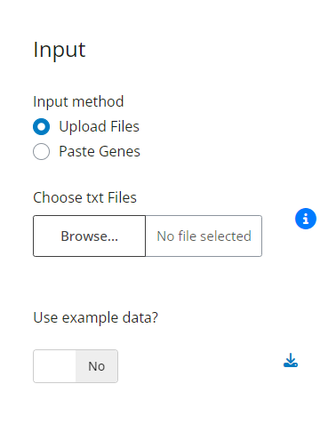
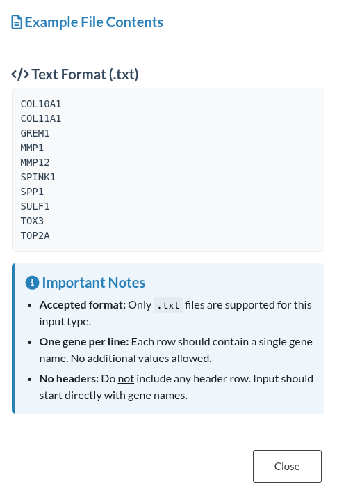
Figure 2: MetaEnrichGO input interface details. (a) Left: MetaEnrichGO input methods panel, allowing selection between file upload or text pasting. (b) Right: Information displayed in the pop-up window ℹ️ regarding the expected example file format.
2.2 Input Example
The table above shows four gene lists used in our example analysis. These lists come from 4 independent studies related to lung cancer and associated with the following identifiers from GEO: GSE10072, GSE19188, GSE63459, GSE75037. Each column corresponds to a list, containing 256, 257, 256 and 236 gene identifiers respectively, including duplicate or missing entries. This arrangement allows direct comparison of the size and composition of the lists across studies, highlighting the diverse scope of each dataset prior to subsequent meta-analysis.
Table 1: Example Data Overview. Combined display of the gene lists from the four lung cancer studies used to demonstrate the analysis workflow.
3 Parameters
Once the gene lists are loaded, six parameters become available to tailor the analysis. These settings cover everything from filtering which genes are included to defining the meta-analysis method. Each option allows precise control over data pre-processing and statistical aggregation to ensure results match the experimental design.
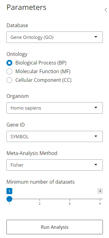
Figure 3: Analysis Configuration Panel. Interface displaying the six adjustable parameters for customizing gene filtering, statistical aggregation, and enrichment settings.
3.1 Database
Gene Ontology (GO): A structured and controlled vocabulary used to describe the functions of genes and their products in a consistent and standardized way. Its content is divided into three sub-ontologies:
- Biological Process (BP): Pathways and larger processes (e.g., cell cycle, signal transduction).
- Molecular Function (MF): Biochemical activities (e.g., ATP binding, kinase activity).
- Cellular Component (CC): Subcellular locations (e.g., nucleus, ribosome).
KEGG (Kyoto Encyclopedia of Genes and Genomes): Database resource for understanding high-level functions and utilities of the biological system, such as the cell, the organism and the ecosystem, from molecular-level information, especially large-scale molecular datasets generated by genome sequencing and other high-throughput experimental technologies.
Reactome: A curated database of human biological pathways and reactions, including signaling, metabolism, and immune system processes. It also supports several model organisms via ortholog mapping.
Personalized: The system allows for the inclusion of customised annotations, provided that they comply with the structure defined in the information section. It is essential to maintain consistency between the nomenclature and the type of input data regarding the employees in the annotation, as automatic matching of identifiers and selection of the organisation is no longer performed. The example file used in this section is available for download and can be reused both for inspection and for future projects.
All four resources serve as the reference background in the Over-Representation Analysis (ORA) step, where the frequency of your input genes in each term or pathway is statistically compared against a genomic background to identify the most significantly enriched biological categories.
3.2 Ontology (GO Only)
When Gene Ontology (GO) is selected as the database, an Ontology choice must be specified. Each GO branch provides a distinct view of gene function:
Biological Process (BP) Describes high-level biological objectives accomplished by ordered assemblies of molecular functions—such as “cell cycle,” “signal transduction,” or “immune response.” Use
BPto discover which overarching pathways or processes your genes collectively influence.Molecular Function (MF) Captures the elemental activities of proteins or gene products at the biochemical level—examples include “ATP binding,” “kinase activity,” or “transcription factor binding.”
MFis ideal for pinpointing the specific enzymatic or binding roles enriched in your gene set.Cellular Component (CC) Defines where gene products exert their function within the cell, such as “nucleus,” “mitochondrion,” or “ribosome.”
CChelps reveal the subcellular localization patterns common to your genes, indicating, for instance, whether they cluster in particular organelles.
Selecting the appropriate ontology refines the enrichment analysis, focusing it on either broader process-level insights (BP), detailed activity-level functions (MF), or spatial context within the cell (CC).
3.3 Personalized File Upload (Personalized database only)
This upload modal provides functionality for importing personalized annotation files. It is accompanied by an information button outlining the required structure and a download button that allows retrieval of the example file in .txt format.
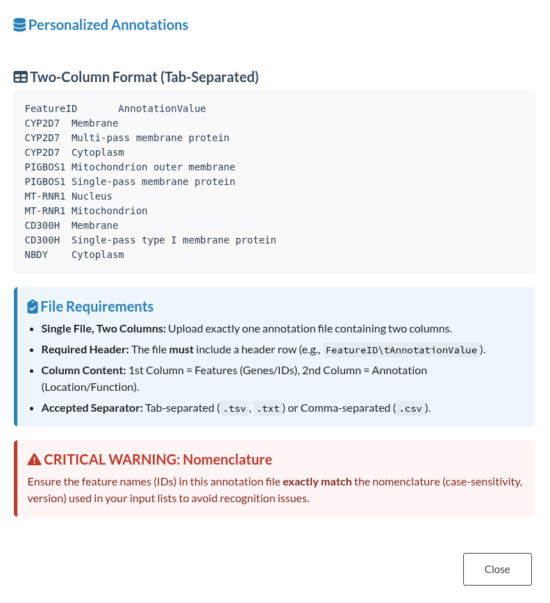
Figure 4: Custom Annotation Upload Interface. Information modal displaying the required file format specifications and providing a downloadable example template.
The example below presents the personalized annotation file used in this case:
Table 2: Example Custom Annotation Dataset. Preview of the ‘protein_location’ file structure used to demonstrate the import of personalized functional annotations.
3.4 Organism (Not available for Personalised)
The following organisms are supported, each identified by an internal code and NCBI Taxonomy ID:
- Homo sapiens (
Hsa; Taxonomy ID: 9606) – Human gene symbols follow the HGNC standard (e.g.,TP53). - Mus musculus (
Mmu; Taxonomy ID: 10090) – Mouse gene symbols use the MGI nomenclature (e.g.,Trp53). - Rattus norvegicus (
Rno; Taxonomy ID: 10116) – Rat gene symbols use RGD notation (e.g.,Rps6kb1).
3.5 Gene ID Type (Not available for Personalised)
Specify the identifier system for your gene lists:
- SYMBOL: Common gene names or symbols (e.g.,
BRCA1). - ENTREZID: Unique numerical IDs assigned by NCBI (e.g.,
672). - ENSEMBL: Stable gene IDs from the Ensembl database (e.g.,
ENSG00000012048).
Warning
Ensuring consistency between the gene list format and the selected identifier type is critical. An incorrect choice of identifier system will result in erroneous mappings and inaccurate enrichment analyses. This constraint applies to all databases except Personalized, where the responsibility for maintaining compatibility rests with the user.
3.6 Meta-Analysis Method (Available if two or more lists are provided)
This parameter determines how p-values from multiple gene enrichment results are statistically combined into a single meta-analytic value. Four established methods are available, each based on different mathematical principles and assumptions:
- Fisher’s Method This technique aggregates independent p-values by calculating the statistic \(-2 \sum \ln(p_i)\) which follows a chi-squared distribution with 2n degrees of freedom (n = number of lists).
Fisher’smethod places greater weight on small p-values, making it highly sensitive when even a few studies show strong enrichment. Best suited for detecting strong signals present in a subset of datasets, especially when consistency across all lists is not required. - Stouffer’s Z-Score Method P-values are first transformed into Z-scores (using the inverse normal distribution), then combined as a weighted sum: \(Z = \frac{\sum w_i z_i}{\sqrt{\sum w_i^2}}\) where \(w_i\) corresponds to a study-specific weight (often proportional to sample size). This approach balances contributions across lists and performs well when list sizes or variances differ. Ideal when datasets vary in size or reliability, allowing integration with custom weighting schemes.
- Tippett’s Method The most straightforward of the group,
Tippett’smethod takes the smallest p-value across all lists as the combined statistic. It excels at detecting categories that are extremely significant in even one dataset but is less robust if significance is spread moderately across many lists. Recommended for exploratory analysis focused on discovering standout signals in individual gene lists. - Wilkinson’s Method A generalization of
Tippett’sapproach,Wilkinson’smethod uses the k-th smallest p-value (for a user-specified k) as the test statistic. By choosing different values of k, the analyst can tune sensitivity toward either early extreme values (small k) or broader consistency (larger k). Useful when the goal is to adjust stringency and detect terms supported by a flexible number of datasets.
3.7 Minimum Number of Datasets (Available if two or more lists are provided)
This slider filters out terms that do not appear in a minimum number of input lists. For example, setting this to 2 means only terms enriched in two or more datasets will be retained. Terms that do not meet this criterion are excluded from the final results and are instead displayed in a separate table of excluded terms, allowing for transparent review and optional downstream inspection.
4 Data Visualization
In the sidebar panel, there is also a tab labeled Data Visualization, which provides options to customize various aesthetic aspects of the output. This includes adjusting the number of columns displayed in the result tables, modifying the color schemes used in the plots, and editing axis titles or other graphical elements to better suit the user’s presentation or analysis preferences.
Note
Any configuration or modification carried out within this section affects all tabs generated in the output interface.
4.1 Table Settings
The interface allows selecting and deselecting specific columns from the final result table. This customization enables users to tailor the displayed information to their needs. When using the download buttons, only the currently visible columns will be included in the exported file. For instance, if only the ID and Description columns are selected out of eight possible ones, the downloaded table will contain just those two.
Note
- Filters applied directly within the table interface (e.g., keyword searches such as “cell”) are reflected in the downloaded file too, but it works after running the analysis
- The table listing excluded genes or terms is not customizable—its structure and contents remain fixed for both display and export (full table).
4.2 Plot Settings
This section allows customization of the appearance of enrichment plots to better suit presentation or analysis needs. Several visual parameters can be adjusted:
- Number of terms to show: Defines how many of the top-ranking enriched terms will be displayed in the plot. This helps focus the visualization on the most relevant results.
- Y-axis: Users can choose what appears on the Y-axis—either the
Term ID, theDescription, or a combination of both. When selecting both, the term and its description are shown together, separated by a hyphen (“-”), providing more context for each entry. - Plot Type: Two types of plots are supported:
- Dot plot, which represents each term as a point, usually with size or color indicating significance or gene count.
- Bar plot, where each term is displayed as a bar, useful for comparing absolute or relative values.
- Color Scale: A gradient color scale is applied based on the adjusted p-value (
p.adjust). Users can customize both ends of the color gradient (low and high values) to match their preferred visual style or color scheme. This makes interpretation easier, especially when using consistent color themes across multiple plots. - Text Size: Allows control over the font size used in the plot. Increasing or decreasing this value can help adapt the plot for screens, print, or accessibility preferences.
5 Outputs
The output section automatically generates one tab per uploaded file, along with an additional tab corresponding to the combined meta-analysis (or ORA combined results). If a single file is uploaded, only one tab is displayed; however, when two or more files are provided, the total number of tabs equals the number of uploaded files plus one for the combined analysis. Each tab contains a results table with download options, followed by an adjustable plot that can be exported in multiple formats.
5.1 Results Table
Provides a detailed summary of enriched terms identified across the input gene sets. It supports sorting, column-based filtering, and downloads in both csv and tsv formats. Each row corresponds to a unique enrichment term, with associated statistical and contextual information.
5.1.1 Available columns:
ID: The unique identifier of the enrichment term. For example, GO:0006915 for “apoptotic process” (Gene Ontology), or 05200 for “Pathways in cancer” (KEGG).
Description: A human-readable name or description of the term, providing biological context.
pvalue: The combined raw p-value derived from the selected meta-analysis method (e.g., Fisher, Stouffer, etc.). This value reflects the probability of observing the enrichment by chance.
- Lower values (e.g., < 0.05) suggest stronger statistical significance.
- Higher values imply less confidence in the enrichment.
p.adjust: The adjusted p-value after correcting for multiple comparisons using the
Benjamini–Hochberg False Discovery Rate (FDR)method. This value controls the proportion of false positives.Again, lower values (e.g., < 0.05 or < 0.01) indicate more reliable and statistically significant results. Adjusted values are especially important when analyzing large gene sets, where multiple testing can inflate false positives.
ListCount: Indicates how many of the input gene lists contained the given enrichment term. Higher values suggest the term is consistently enriched across multiple datasets, which can point to broader biological relevance.
ListNames: Lists the names of the input files or datasets in which the term was found. This helps trace back which experiments or conditions contributed to each enrichment.
GeneCount: Total number of genes associated with the term in the datasets where it appeared. Useful to assess the size of the gene set behind the enrichment signal.
GeneID: A list of gene identifiers (
SYMBOL,ENTREZID, orENSEMBL, depending on user selection) that contributed to the enrichment for that term. These are the genes from the input lists that overlapped with the term’s annotation.
Note
Each column in the results table includes a small question mark icon that provides additional information when hovered over. These tooltips offer concise explanations of the column’s purpose and how to interpret its values, allowing users to quickly understand the data without needing to refer back to the documentation. Simply place your cursor over the icon to view the tooltip — no need to click.
When using standard databases like ORA or KEGG, the enrichment results contain the columns GeneID and GeneCount, indicating the genes associated with the identified terms. Conversely, in analyses employing personalized annotations, where the annotated entities may represent various molecular types, these columns are replaced with FeatureID and FeatureCount to enhance interpretability and adaptability.
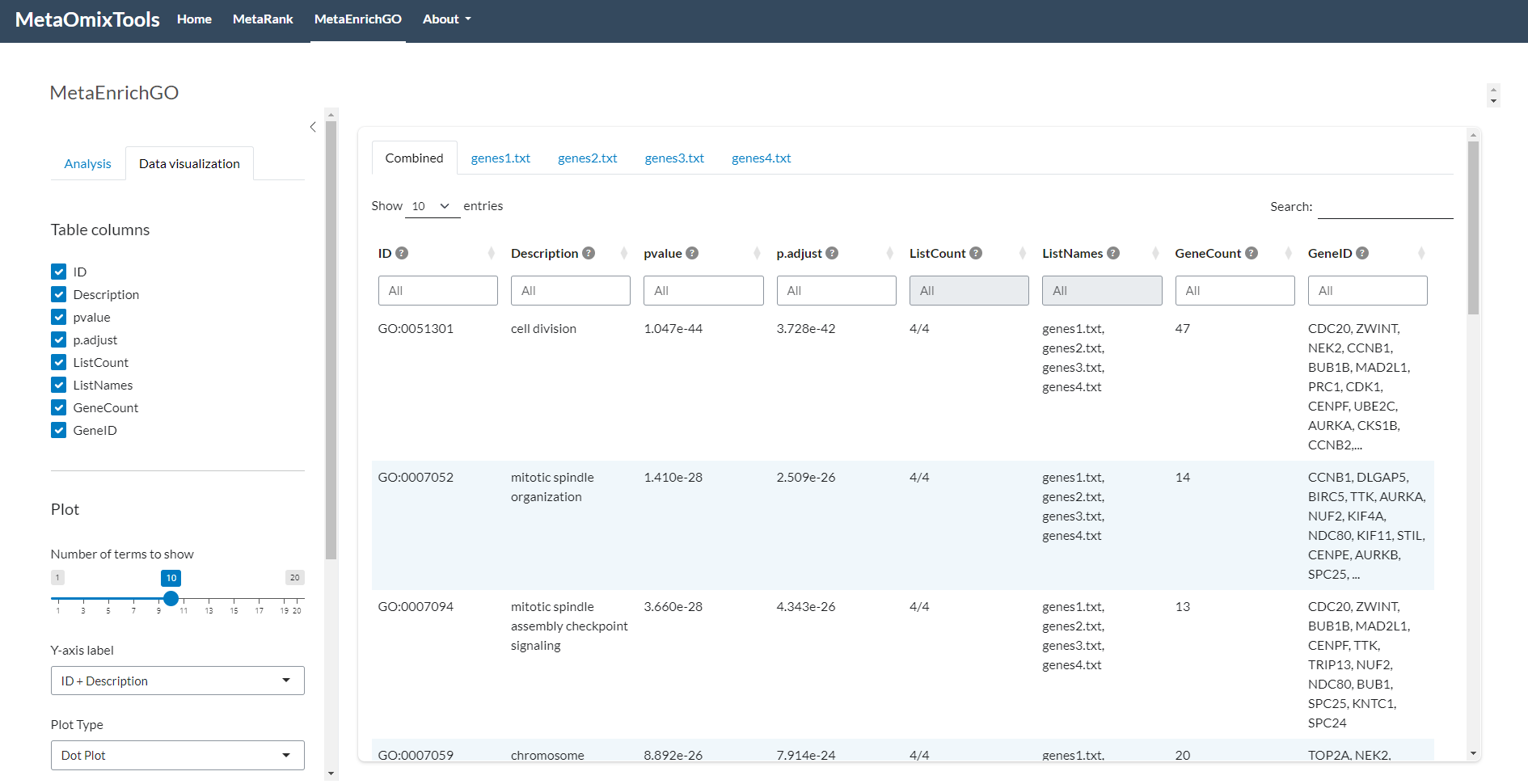
Figure 5: Main Enrichment Results Table. Comprehensive display of the significant terms identified in the analysis, featuring statistical metrics, gene counts, and dataset contributions.
5.1.2 Excluded Terms
A secondary table is available to display enrichment terms that were excluded from the main results due to not meeting the Minimum Number of Datasets threshold. This table is accessible via the eye icon toggle and is intended to provide transparency regarding filtered-out data.
Unlike the main results table, the excluded terms are not subjected to the meta-analysis step, and thus do not contain combined p-values or adjusted p-values. This design choice helps reduce computation time while still allowing users to inspect the removed terms.
The structure of this table differs slightly:
- It includes information such as the term
ID,Description,ListCount,ListNames,GeneCountandGeneID. - Statistical columns such as
pvalue,p.adjust, or plot-related metadata are not included.
The table supports interactive filtering and sorting, but column selection is not available. Downloads are limited to tsv format only, and reflect the entire table contents as displayed (i.e., column visibility cannot be modified).
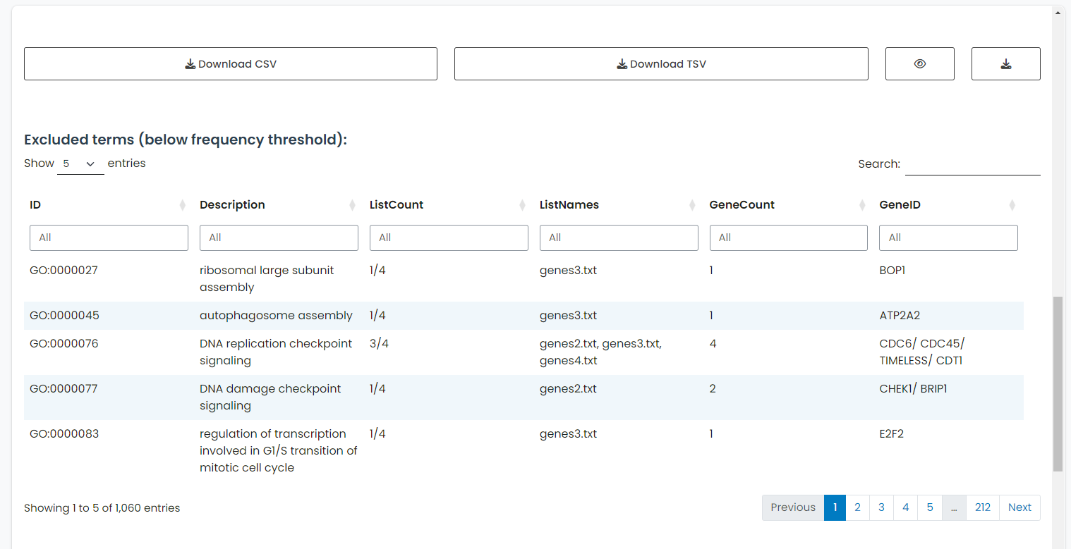
Figure 6: Excluded Terms Table. Secondary view displaying enrichment terms that did not meet the minimum dataset threshold, showing occurrence data without computed statistical metrics.
5.2 Plot Output
The data resulting from the meta-analysis and summarized in the main results table is also represented visually through interactive plots. These plots provide a complementary overview of enriched terms and support intuitive interpretation of the results with this following features:
- Two plot type are available: Dot Plot and Bar Plot, both depicting the number of genes associated with each term (
gene count) and their corresponding adjusted p-values (p.adjust). The color scale can be customized to reflect statistical significance. - Tooltips appear on hover, displaying key information such as the full term or pathway name, GeneCount, and adjusted p-value, enhancing interpretability.
- Download Options include
png,jpg, orhtml(interactive) formats, allowing users to export plots for presentations or further analysis.
Note
Table-Plot reactivity ensures consistency. For example, filtering the results table (e.g., by the word “cell”) dynamically updates the plot to show only the matching terms.
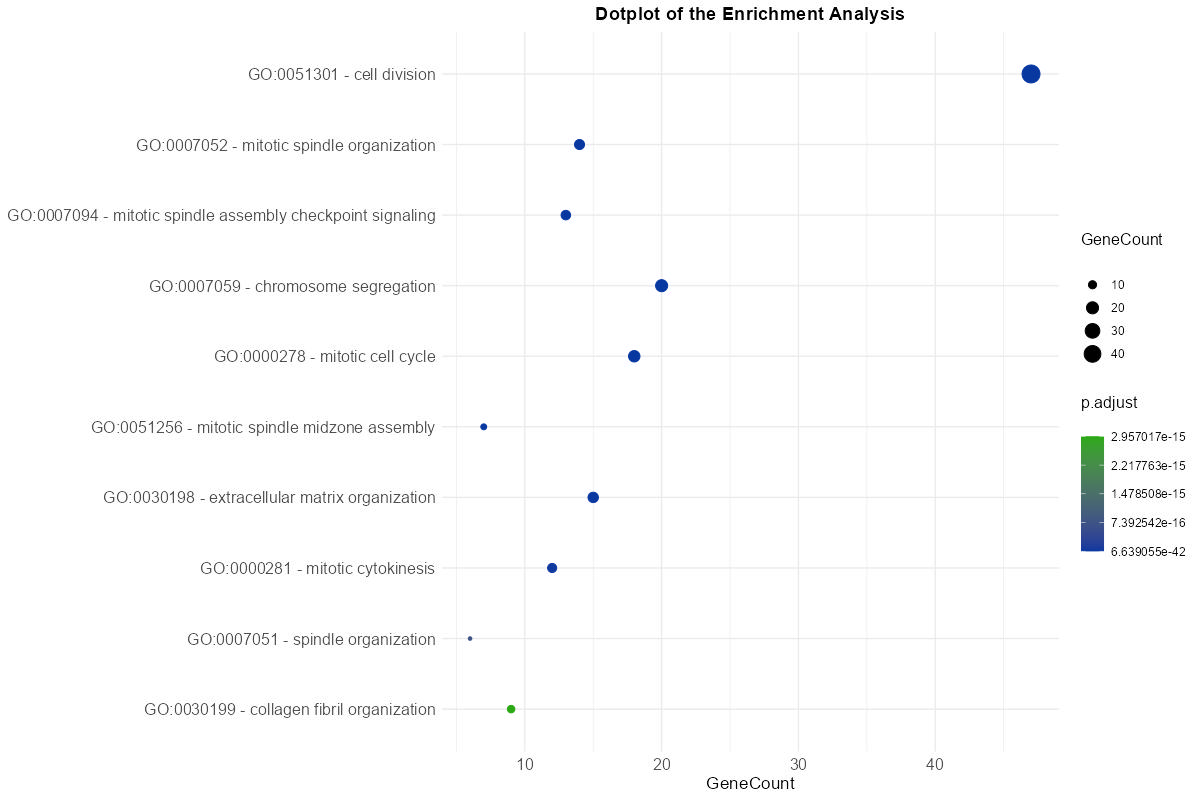
Figure 7: Enrichment Dot Plot. Visualization of significant terms where dot size corresponds to gene count and color indicates statistical significance.
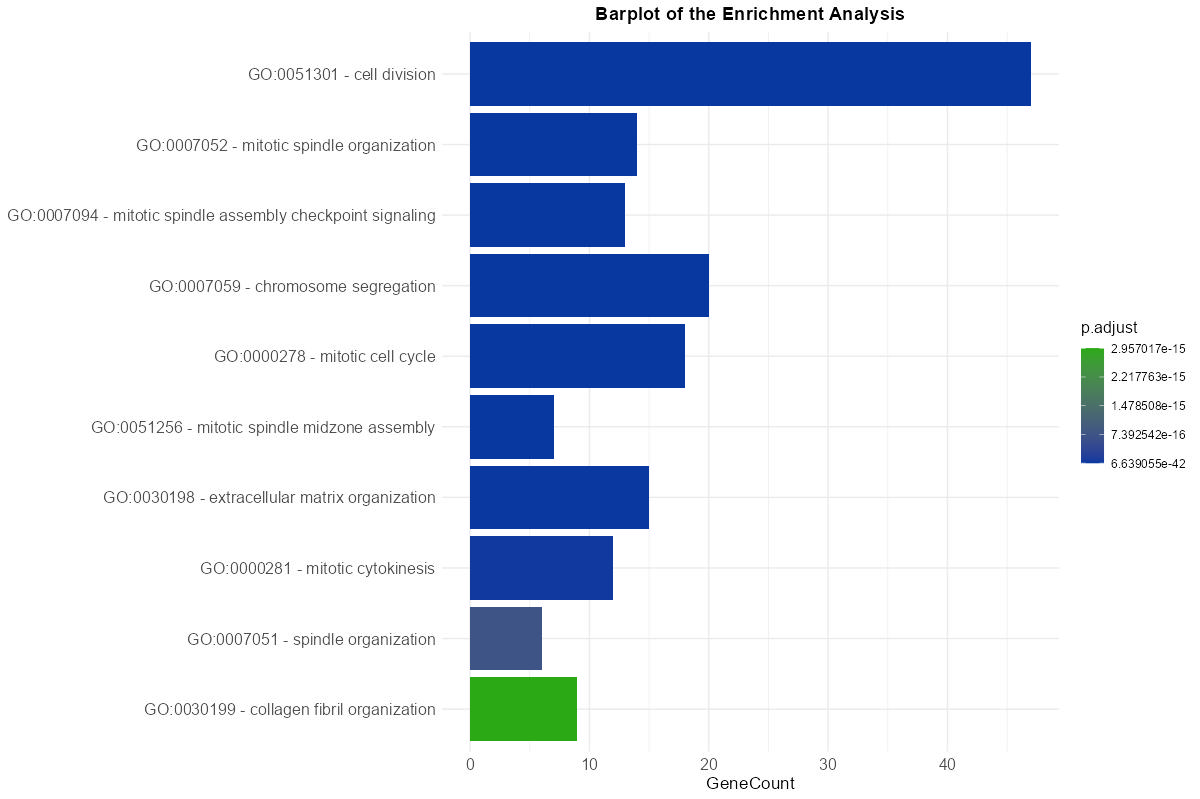
Figure 8: Enrichment Bar Plot. Graphical representation of top enriched terms showing the number of associated genes and their significance levels.
6 Background Pipeline
The MetaEnrichGO workflow processes input gene lists through a structured, reactive pipeline designed to ensure data integrity before performing statistical analysis and visualization. The internal logic operates as follows:
Data Ingestion and Validation
- Input Parsing: The system accepts inputs via file upload (
.txt,.tsv) or direct text pasting. File inputs are read line-by-line, trimming whitespace and discarding empty lines. Pasted text is tokenized using the###delimiter to distinguish between multiple lists. - Strict Validation: Before analysis, inputs undergo a rigorous check via custom functions (
validate_file_format,validate_gene_ids,validate_organism). This step detects forbidden characters (e.g., hidden tabs from Excel), verifies gene ID formats (SYMBOL/ENTREZ/ENSEMBL) using Regular Expressions, and ensures nomenclature matches the selected organism (e.g., uppercase for Human vs. title case for Mouse) . - Mapping Check: A preliminary mapping verification ensures that the provided identifiers exist in the selected database, preventing the analysis of meaningless data .
- Input Parsing: The system accepts inputs via file upload (
Annotation Retrieval and ORA
- Offline Enrichment: Instead of relying on API-dependent functions (like
enrichGO), the system utilizes the genericenricher()function fromclusterProfiler. It loads pre-processed annotation objects (containingTERM2GENEandTERM2NAMEdataframes) directly from the local/database_annotations/directory. This approach ensures speed and stability, allowing the tool to function without internet dependency. - Standardization: The raw outputs from the Over-Representation Analysis (ORA) are standardized. If the database is “Personalized”, columns are dynamically renamed (e.g.,
FeatureIDreplacesGeneID) to maintain consistency across the UI.
- Offline Enrichment: Instead of relying on API-dependent functions (like
Meta-Analysis of P-Values
- Intersection Filtering: To optimize performance, the algorithm first calculates term frequency across all datasets. Terms that do not meet the user-defined “Minimum number of datasets” threshold are immediately segregated into an “Excluded” set, avoiding unnecessary statistical computation.
- Statistical Combination: For the remaining “Included” terms, raw p-values are extracted from each contributing study and combined using the selected method (
Fisher,Stouffer,Tippett, orWilkinson). - Adjustment: A final p-value adjustment is applied to the combined results using the Benjamini–Hochberg procedure to control the False Discovery Rate (FDR).
Dynamic Result Presentation
- Tabular Generation: The system dynamically generates a “Combined” results tab along with individual tabs for each input list. The tables utilize custom JavaScript callbacks to render hover tooltips for column headers and format long gene lists for readability.
- Visualization: Interactive Dot plots and Bar plots are generated using
ggplot2and converted toplotlyobjects. These visual components are fully reactive, updating in real-time based on table filtering and user-selected thresholds (e.g., top N terms, color gradients). - Export Options: Results are available for download in multiple formats, including raw data tables (
csv,tsv) and high-resolution plots (png,jpg,html), with specific handling for “Excluded” terms which are downloadable separately.
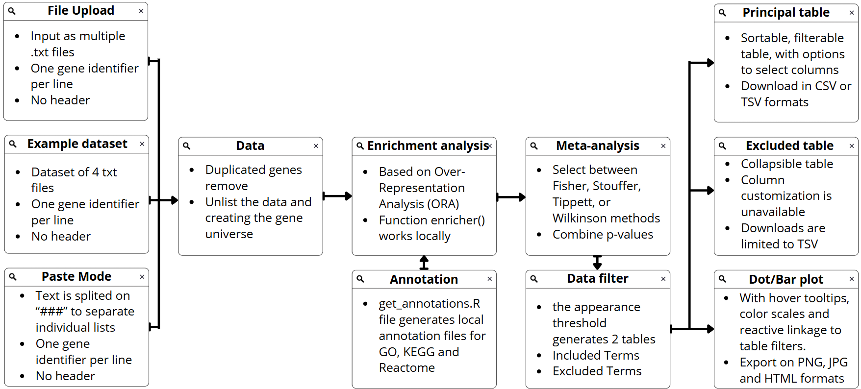
Figure 9: MetaEnrichGO Analysis Pipeline. Schematic overview of the four-stage workflow, detailing the process from data ingestion and strict validation to statistical meta-analysis and interactive visualization.
7 Best Practices
Ensure correct input formatting. Input files should list one gene identifier per line without headers. While the system automatically handles consistent line endings (Unix or Windows ), adhering to a clean, single-column text format simplifies pre-processing and prevents parsing errors.
Match identifier type and organism code. Verify that your gene IDs (
SYMBOL,ENTREZID, orENSEMBL) strictly correspond to the selected organism (e.g., Hsa for human, Mmu for mouse). Mismatches—such as using uppercase human symbols for mouse data—will lead to failed mappings and valid genes being discarded during validation.Prepare custom annotation files carefully. When using the “Personalized” database option, your annotation file must contain exactly two columns (
Feature IDandDescription) with a header row. Crucially, the feature IDs in your input lists must match the IDs in this annotation file exactly (case-sensitive) to ensure successful mapping.Leverage example datasets. Use the built-in example files to familiarize yourself with the required structure. Loading these before running your own data helps validate that the tool is functioning correctly and allows you to test different parameter settings without errors.
Select the meta-analysis method to suit your study design.
- Use
FisherorTippettwhen seeking strong signals that may be present in only a subset of your gene lists. - Choose
StoufferorWilkinsonfor a more balanced integration when comparing datasets of variable sizes or quality.
- Use
Adjust the minimum dataset threshold thoughtfully. Setting a high threshold increases confidence by highlighting terms consistently enriched across many lists, but it may exclude potentially relevant biological categories present in only a few. Conversely, lower thresholds increase sensitivity but may raise the false positive rate.
Navigate results tabs effectively. Distinguish between the analysis levels: the “Combined” tab displays the integrated meta-analysis results, while the subsequent individual tabs (e.g.,
"List1","List2") show the independent Over-Representation Analysis (ORA) results for each specific dataset. Reviewing individual tabs is useful for tracing the origin of a combined signal.Review excluded terms. If a term of particular interest is missing from the main results, consult the “Excluded Terms” table (available in the Combined tab). This table reveals terms that were statistically significant but failed to meet the “Minimum number of datasets” appearance filter.
Customize visualization settings for clarity. Adjust table columns, plot type, color scales, and font sizes to enhance readability and highlight key findings in presentations or publications.
Monitor performance. Very large numbers of input lists (e.g., >30 lists) or an excessive number of enriched terms (>1000) can slow down the interactive plotting. In such cases, consider reducing the number of input lists, narrowing the “Number of terms to show” slider, or increasing the filtering threshold to improve responsiveness.
8 Troubleshooting
| Issue | Possible Solution |
|---|---|
| Absent Input Data | The user has not provided any type of file or pasted information in the input option used to perform the analysis. The system requires valid input to initiate any process. |
| Absent Annotation File | When selecting a “Personalized” database, a custom annotation file is mandatory. The analysis will stop if the “Choose annotation file” field is left empty. |
| File Format Error | Input files must be in plain text (.txt). Common errors include the presence of commas (,), tabs (\t), semicolons (;), or hash symbols (#). Ensure the file contains only one gene per line and has no headers or hidden formatting. |
| Paste Format Error | When using “Paste Genes”, ensure the data does not contain hidden formatting from Excel or separators like tabs or commas. If pasting multiple lists, they must be separated strictly by a line containing ###. |
| Invalid Organism | Gene nomenclature must match the selected organism. For example, Homo sapiens genes typically use all uppercase (e.g., TP53), while Mus musculus uses title case (e.g., Trp53). Mismatches here will block the analysis. |
| Invalid Gene Identifiers | This error occurs when the gene IDs do not match the selected type (SYMBOL, ENTREZID, ENSEMBL). If the error rate exceeds 50%, the analysis stops. For minor mismatches, a warning allows you to continue. |
| No Significant Results | If no terms appear after enrichment analysis, the issue often lies in overly strict filters or insufficient overlap across datasets. One key parameter to review is the “Minimum Number of Datasets” threshold; if it’s set too high, many terms may be excluded. Consider lowering this threshold to include more terms. Also ensure that gene lists have enough common genes to detect shared biological processes. |
| Gene Mapping Failure | The input format is technically valid (clean text), but the provided genes do not exist in the selected database. This often happens when using “fake” gene names or incorrect IDs that cannot be mapped. |
| Slow Performance | Performance can be significantly impacted by the size and number of input datasets. Increasing the dataset threshold can help by filtering out less relevant terms. In general, avoid uploading or pasting excessively large datasets unless necessary for your analysis. |
| Annotation File Format | Custom annotation files must contain exactly two columns. The system validates this structure and will reject files that do not strictly adhere to the Feature ID and Annotation Value format. |
Table 3: Troubleshooting Guide. Summary of common validation errors, their potential causes, and suggested solutions to ensure successful analysis execution.
In addition to the summarized issues and suggestions presented in the table above, the following section visually illustrates the main error messages that may appear during the use of the application. Each message corresponds to a common input or processing issue, offering a brief explanation of what went wrong, how it affects the workflow, and what can be done to resolve it. In some cases, specific files or pieces of information that caused the problem are clearly indicated to help the user correct the input efficiently and continue without interruption.
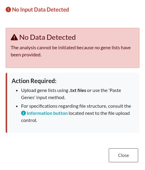
Figure 10: Missing Input Data. Alert modal triggered when an analysis is attempted without providing any gene lists or valid input files.
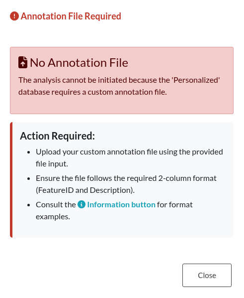
Figure 11: Missing Annotation File. Error message displayed when the ‘Personalized’ database option is selected but the required custom annotation file has not been uploaded.
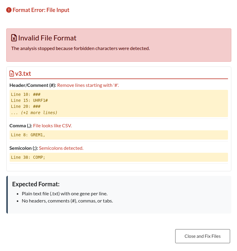
Figure 12: File Format Validation Error. Alert displayed when uploaded files contain headers, incorrect delimiters, or unsupported file types that prevent parsing.
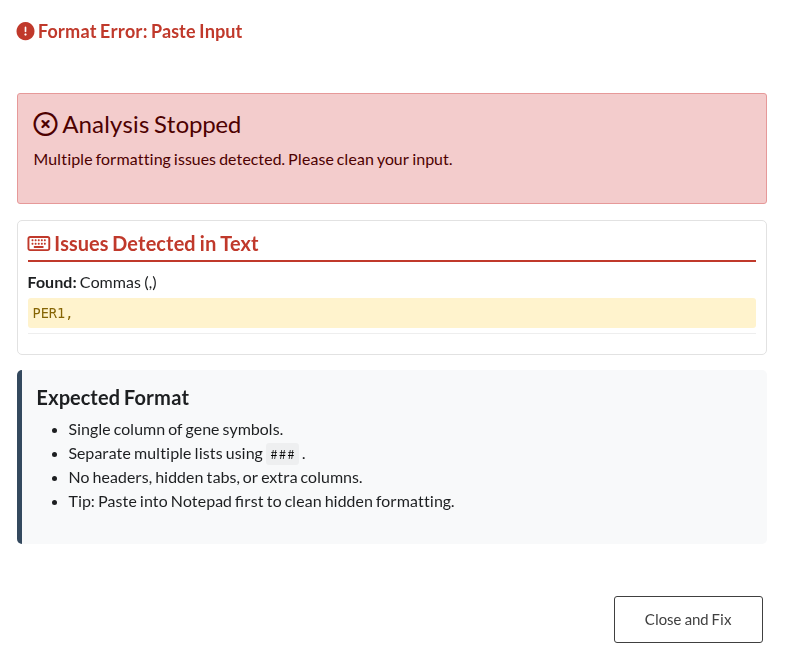
Figure 13: Paste Input Formatting Error. Validation alert indicating issues with pasted text, such as missing delimiters (###) between lists or empty content.
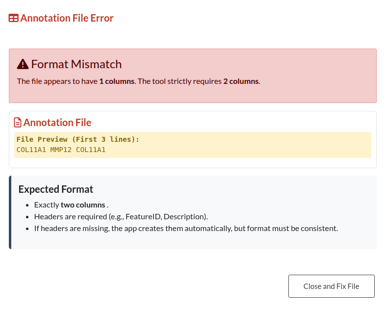
Figure 14: Annotation Structure Error. Validation modal triggered when the uploaded custom annotation file does not adhere to the required two-column format.
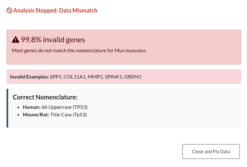
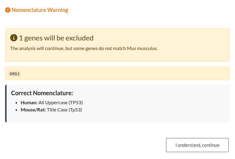
Figure 15: Validation outcomes for Gene IDs and Organism nomenclature. (a) Left: “Analysis Stopped” (Red Modal). This occurs when the error rate exceeds 50%, blocking the analysis until the input or parameters are corrected. (b) Right: “ID Format Warning” (Orange Modal). This occurs when a minority of IDs are incorrect (<50%), allowing the user to ignore the mismatched genes and continue the analysis.
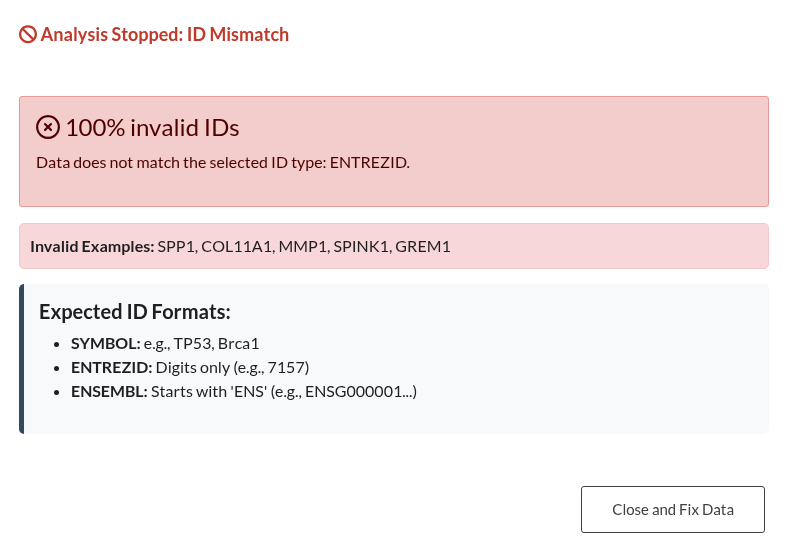
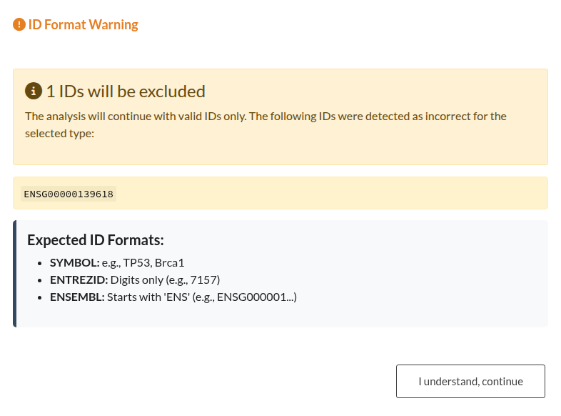
Figure 16: Validation outcomes for Gene IDs. (a) Left: “Analysis Stopped” (Red Modal). This occurs when the error rate exceeds 50% (e.g., using Ensembl IDs when “SYMBOL” is selected), blocking the analysis until the input or parameters are corrected. (b) Right: “ID Format Warning” (Orange Modal). This occurs when a minority of IDs are incorrect (<50%), allowing the user to ignore the mismatched genes and continue the analysis.
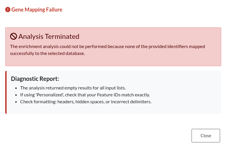
Figure 17: Database Mapping Failure. Error modal indicating that while the input text is valid, none of the provided gene identifiers could be mapped to the selected functional database.
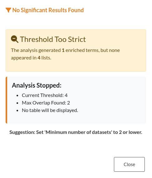
Figure 18: Empty Result Set. Notification advising the user to relax filtering parameters (such as the minimum number of datasets) after the analysis yielded no significant enrichment terms.